How to use VLOOKUP in Excel to join data from a tab separated export

This is probably the most popular formula I use to link up tables of data. Click here to view a video tutorial about using VLOOKUP

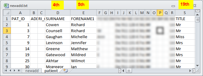
99% of the exported Vision data will always show the PAT_ID in the first column. This is the link that joins all the data together.

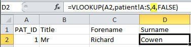
The formula looks something like this: =VLOOKUP(A2,patient!A:S,19,FALSE)

• A2 is the patient ID to use as the lookup in the other table of data. Therefore, the PAT_ID must exist in both spreadsheets, and it is the starting point of the search.
• patient! is the other spreadsheet name that holds the data you want
• A:S is the table of data on this spreadsheet. The table must start from PAT_ID (i.e. column A) and include the column of data you want to show - in this case anything between column A and column S means I will be able to show the data from any column within this range.
• 19 is the 19th column starting from column A that holds the data I want displayed
• FALSE has to find the exact PAT_ID to be a match.
  Whereas TRUE gives an approximate match, so if the value you're looking up is not found in the list it uses the nearest it can find without going over.

Notice that the majority of the formula will remain the same because the forename and surname columns are within A:S, which means I only need to change the column number in the formula.